Driving the simulator – data and software

If we want to do a realistic traffic simulation, we can’t just set up a bunch of long FTP downloads. Real-world traffic is a mix of mostly short and very few long TCP flows, with a good dollop of UDP and some ICMP thrown in for good measure. Short TCP flows never live long enough on satellite links to experience the effects of TCP flow control: They often consist of only one or two packets, and by the time the first ACK gets back to the sender, the sender has already sent everything. So if we want to recreate that scenario, we need to gather some intelligence about real traffic first.

One way to do this is to go to a friendly ISP in an island location and collect netflow traces at their border router to the satellite gateway. One caveat here is to ensure that we’re responsible citizens: Raw netflow traces are huge files even for just a few minutes worth of traffic. Trying to retrieve them via the satellite link is a surefire way of making yourself unpopular on the island. It’s a bit like a surgeon gaining access to your abdomen via keyhole surgery, and then trying to pull your liver out through the hole in one piece. Not smart. So the secret is to keep the traces short and at the very least compress them. Even better: Store the data on a portable drive and physically retrieve it from the island.

An analysis of netflow traces gives us an idea of how flow sizes are distributed. The two diagrams show an example of what one may observe: Most TCP flows are small, but most of the bytes transferred belong to large flows. So if TCP queue oscillation puts TCP senders of large flows into a start-stop mode of operation but leaves small flows almost unaffected, then it still puts the brakes on the majority of bytes travelling across the link.

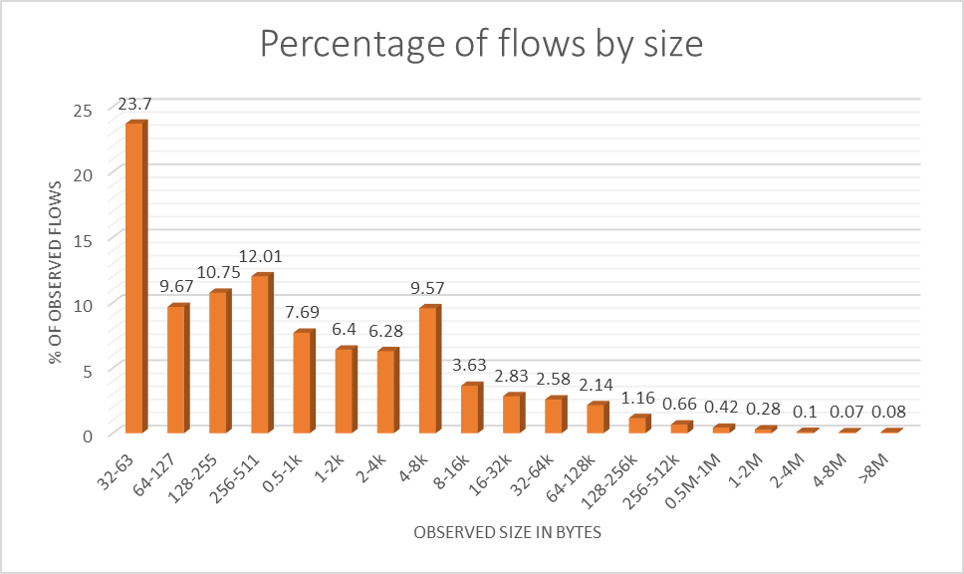
The vast majority of flows is so small that they will fit into just a couple of IP packets each.

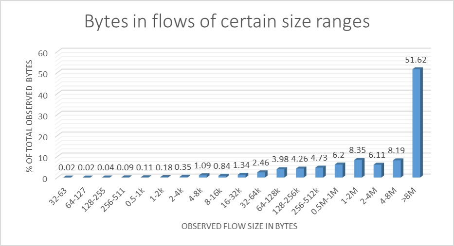
However, most of the data on satellite links is contributed by really large flows.

To give you a bit of an idea as to how long the tail of the distribution is: We’re looking at a median flow size of under 500 bytes, a mean flow size of around 50 kB, and a maximum flow size of around 1 GB.

A quick reminder for those who don’t like statistics: The median is what you get if you sort all flows by size and take the flow size half-way down the list. The mean is what you get by adding all flow sizes and dividing by the number of flows. A distribution with a long tail has a mean that’s miles from the median. Put simply: Most flows are small but most of the bytes sit in large flows.

Simulating traffic: Supplying a controllable load level

Another assumption we make is this: By and large, consumer Internet users are reasonably predictable creatures, especially if they come as a crowd. As a rule of thumb, if we increase the number of users by a factor of X, then we can reasonably expect that the number of flows of a particular size will also roughly increase by X. So if the flows we sampled were created by, say, 500 users, we can approximate the behaviour of 1000 users simply by creating twice as many flows from the same distribution. This gives us a kind of “load control knob” for our simulator.

But how are we creating the traffic? This is where our own purpose-built software comes in. Because we have only 84 Pis and 10 NUCs, but want to be able to simulate thousands of parallel flows, each physical “island client” has to play the role of a number of real clients. Our client software does this by creating a configurable number of “channels”, say 10 or 30 on each physical client machine.

Each channel creates a client socket, randomly selects one of our “world” servers to connect to, opens a connection and receives a certain number of bytes, which the server determines by random pick from our flow size distribution. The server then disconnects, and the client channel creates a new socket, selects another server, etc. Selecting the number of physical machines and client channels to use thus gives us an incremental way of ramping up load on the “link” while still having realistic conditions.

Simulating traffic: Methodology challenges

There are a couple of tricky spots to navigate, though: Firstly, netflow reports a significant number of flows that consist of only a single packet, with or without payload data. These could be rare ACKs flowing back from a slow connection in the opposite direction, or be SYN packets probing, or…

However, our client channels create a minimum amount traffic per flow through their connection handshake. This amount exceeds the flow size of these tiny flows. So we approximate the existence of these flows by pro-rating them in the distribution, i.e., each client channel connection accounts for several of these small single packet flows.

Secondly, the long tail of the distribution means that as we sample from it, our initial few samples are very likely to have an average size that is closer to the median than to the mean. In order to obtain a comparable mean, we need to run our experiments for long enough so that our large flows have a realistic chance to occur. This is a problem in particular with experiments using low bandwidths, high latencies (GEO sats), and a low number of client channels.

For example, a ten minute experiment simulating a 16 Mbps GEO link with 20 client channels will typically generate a total of only about 14,000 flows. The main reason for this is the time it takes to establish a connection via a GEO RTT of over 500 ms. Our distribution contains well over 100,000 flows, with only a handful of really giant flows. So results at this end are naturally a bit noisy, depending on whether, and which, giant flows in the 100’s of MB get picked by our servers. This forces us to run rather lengthy experiments at this end of the scale.

Simulating the satellite link itself

For our purposes, simulating a satellite link mainly means simulating the bandwidth bottleneck and the latency associated with it. More complex scenarios may include packet losses from noise or fading on the link, or issues related to link layer protocol. We’re dedicating an entire server to the simulation (server K in the centre of the topology diagram), so we have enough computing capacity to handle every case of interest. The rest is software, and here the choice is chiefly between a network simulator (such as, e.g., sns-3) and something relatively simple like the Linux tc utility.

The latter lets us simulate bandwidth constraints, delay, sporadic packet loss and jitter: enough for the moment. That said, it’s a complex beast, which exists in multiple versions and – as we found out – is quite quirky and not overly extensively documented.

Following examples given by various online sources, we configured a tc netem qdisc to represent the delay, which we in turn chained to a token bucket filter. The online sources also suggested quality control: ping across the simulated link to ensure the delay is place, then run iperf in UDP mode to see that the token bucket filter is working correctly. Sure enough, the copy-and-paste example passed these two tests with flying colours. It’s just that we then got rather strange results once we ran TCP across the link. So we decided to ping while we were running iperf. Big surprise: Some of the ping RTTs were in the hundreds of seconds – far longer than any buffer involved could explain. Moreover, no matter which configuration parameter we tweaked, the effect wouldn’t go away. So, a bug it seemed. We finally found a workaround involving ingress redirection to an intermediate function block device, which passed the tests and produced what seemed to be sensible results for TCP. Just goes to show how important quality control is!

In late 2020, we discovered that even this level of quality control had not been enough. An upgrade to Ubuntu 20.04 broke tc and suddenly failed this test in most cases, with swathes of packets lost early on in its operation, a condition that either then disappeared or persisted until the tc elements were removed and reintroduced. Trying to figure out whether it was the test tools that had failed or the tc arrangement, we wrote a dedicated link testing software.

Four phase link testing

The new software runs a four-stage process to test the link that uses sequence numbered and padded UDP packets with timestamps that the test client sends to a server at the far end of the link. The server returns the packets to the client, without padding so as not to load the return link more than absolutely need be.

In the first of the four stages, the software feeds the emulated link at (just below) its nominal rate. In reality, we would expect this to result in a bare-bones round-trip-time (RTT) and at
best sporadic packet loss (in the absence of background traffic). The client tests for that by checking whether any sequence numbers failed to return and whether any of these takes significantly longer than the pure link round-trip time configured on the emulator. A link that passes this test stage has at least the nominal capacity and the correct bare-bones RTT.

In the second stage, we continue at this feed rate but add a burst of packets designed to (almost) fill the link’s input buffer, something the iperf3 and ping test could not do. In theory, we expect this to result in an RTT that’s bare bones plus the input buffer’s queue sojourn time, again with only negligible packet loss. If the link passes this stage, we know that the input buffer size is at least what we have configured, as any smaller buffers would overflow and produce packet loss and result in a shorter RTT.

Stage three of the test continues seamlessly at the same feed rate, but at this point, the input buffer is practically full – the link drains it at the same rate as the feed replenishes it. Another burst of the same size as in the second stage now makes the buffer overflow. This should result in packet loss approximately equivalent to the size of the burst, while the RTT should remain unchanged over stage 2. If the link passes this stage, we know that the input buffer size is at most what we want. We can also be confident that there are no hidden bottleneck buffers in the system that we don’t know about as these would absorb packets without dropping them, while increasing the RTT.

Stage 4 ramps up the feed rate to 10% above nominal and looks for ~10% packet loss at unchanged RTT. If a link passes this stage, we know that it has at most the nominal capacity.

We then tested this on our tc-based emulations. They always failed stage 2 and 3 of the test wholesale, even when it passed the original test. In other words, the emulation got the rate right, it got the delay right, but it didn’t deal with bursts the way we would expect it from a true bottleneck. This looked like a rubber bottleneck!

To an extent, we had been aware of this. The token bucket filters in Linux are designed to assist in restrict bandwidth to users and require a “burst” link rate to be set in addition to the nominal rate. In other words, they cap the average rate to a peak but not the instantaneous rate. However, we had kept the difference to a small amount and so did not consider this to be a likely source of problems. Not so as it would turn out.

With our previous link emulation clearly not usable, we needed a Plan B, however, so set upon building a userland link emulator.

The userland link emulator

To build the userland link emulator, we were able to leverage the existing titrator codebase, which already contained a custom token bucket filter very similar to the one needed in the link emulator. It also contained queueing code that could easily be extended to yield a delay queue, meaning the userland link emulator did not take long to develop. Having the new testing tool at hand as well as the existing tests was an added bonus.

After extensive testing, we can now confirm that we are able to emulate GEO links across our entire “poster child” range and MEO links up to 160 Mb/s, with the emulated links passing the tests with flying colours. This currently only leaves us stranded for our 320 Mb/s MEO simulations, for which the emulator is not quite fast enough. We have identified potential for further acceleration, but this will have to wait as it requires significant code refactoring in the packet acquisition routine.

The big surprise then came when we repeated our baselines: Across the board, goodput over the new links was significantly worse than under the tc-based emulator. This was not a bug in the emulator, however, but a result of denying link entry to bursts: When we then tried coded traffic across the same link emulation, we achieved significantly more goodput – multiple times the baseline at low loads, in fact. This behaviour was much closer to what we had seen in the field.

Lesson learned: It is well known that large buffers on satellite links increase goodput (see Background and Justification section) by absorbing traffic bursts above the nominal rate. Our tc-based emulator clearly did the same and a bit more by allowing such bursts to enter the link without increasing the queue sojourn time.

Simulating world latency

We also use a similar technique to add a variety of fixed ingress and egress delays to the “world” servers. This models the fact that TCP connections in real life don’t end at the off-island sat gate, but at a server that’s potentially a continent or two down the road and therefore another few dozen or even hundreds of milliseconds away.

Link periphery and data collection

We already know that we’ll want to try PEPs, network coders etc., so we have another two servers each on both the “island” (servers sats-pepi and sats-codi) and the “world” (servers sats-codw and sats-pepw) side of the server sats-em that takes care of the “satellite link” itself. Where applicable, these servers host the PEPs and / or network coding encoders / decoders. Otherwise, these servers simply act as routers. Note that if we wish to both code and PEP, the coded tunnel needs to go between the PEP machines and not across the PEP link. Together, sats-pepi, sats-codi, sats-em, sats-codw and sats-pepw make up the “satellite link chain”.

Between all of the servers along the satellite link chain, as well as on the island side of sats-pepi and the world side of sats-pepw, all traffic passes through Viavi copper taps which function as our observation points and make phyiscal copies of all traffic heading to the island side. Each of these copper taps feeds into one of two capture servers (sats-ci and sats-cw), where we run tcpdump to capture the packets and log them into pcap capture files.

An alternative to data capture here would be to capture and log on the clients and / or “world” servers. However, capture files are large and we expect lots of them, and the SD cards on the Raspberry Pis really aren’t a suitable storage medium for this sort of thing. Besides that, we’d like to let the Pis and servers get on with the job of generating and sinking traffic rather than writing large log files. Plus, we’d have to orchestrate the retrieval of logs from over 130 machines with separate clocks, meaning we’d have trouble detecting effects such as link underutilisation.

So the copper taps are really without a lot of serious competition as observation points. After each experiment, we use tshark to translate the pcap files into text files, which we then copy to our storage server (bottom).

For some experiments, we also use other tools such as iperf (so we can monitor the performance of a well-defined individual download) or ping (to get a handle on RTT and queue sojourn times). We run these between the NUCs and some of the more powerful “world” servers.

A basic experiment sequence

Each experiment basically follows the same sequence, which we execute via our core script:

1. Configure the “sat link” with the right bandwidth, latency, queue capacity etc.
2. Test the “sat link”.
3. Configure and start any network coded tunnel we wish to use between servers sats-codw and sats-codi, with or without titration.
4. Configure and start any PEP we wish to use between servers sats-pepw and sats-pepi.
5. Test the reachability of all interfaces that should be pingable.
6. Start the tcpdump capture at the island end (server sats-ci) of the link.
7. Start the tcpdump capture at the world end (server sats-cw) of the link with a little delay. This ensures that we capture every packets heading from the world to the island side.
8. Start the iperf3 server on one of the NUCs. Note that in iperf, the client sends data to the server rather than downloading it.
9. Reset the path MTU (PMTU) cache on the world server machines.
10. Start the world servers.
11. Ping the special purpose Pi on the island side from the special purpose Pi on the world side. This functions as a kind of “referee’s start whistle” for the experiment as it creates a unique packet record in all tcpdump captures, allowing us to synchronise them later.
12. Start the island clients as simultaneously as possible.
13. Start pinging from sats-ping to the island side – typically, we ping 10 times per second.
14. Start an iperf3 transfer from sats-sp to the NUC from step 6 for half of the core experiment duration.
15. Wait for the core experiment duration to expire. The clients terminate themselves.
16. Ping the special purpose client from the special purpose server again (“stop whistle”).
17. Terminate pinging (usually, we ping only for part of the experiment period, though)
18. Terminate the iperf client.
19. Terminate the iperf server.
20. Terminate the world servers.
21. Convert the pcap files on sats-ci and sats-cw into text log files with tshark
22. Retrieve text log files, iperf log and ping log to the storage server.
23. Start the analysis on the storage server.

Between most steps, there is a wait period to allow the previous step to complete. For a low load 8 Mbps GEO link, the core experiment time needs to be 10 minutes to yield a half-way representative sample from the flow size distribution. The upshot is that the pcap log files are small, so need less time for conversion and transfer to storage. For higher bandwidths and more client channels, we can get away with shorter core experiment durations. However, as they produce larger pcap files, conversion and transfer take longer. Altogether, we budget around 20 minutes for a basic experiment run.

Tying it all together

We now have more than 100 machines in the simulator. Even in our basic experiments sequence, we tend to use most if not all of them. This means we need to be able to issue commands to individual machines or groups of machines in an efficient manner, and we need to be able to script this.

Enter the parallel-ssh utility. This useful little program lets our scripts establish a number of SSH connections to multiple machines simultaneously, e.g., to start our servers or clients, or to distribute configuration information. This lets us start up all client machines within typically less than a second.

Automating the complex processes is vital, so we keep adding scripts to the simulator as we go to assist us in various aspects of analysis and quality assurance.